wav-nn: Generating wav files with a neural network

Introduction Link to heading

This post is about a project to generate wav files with a neural network. These are files with the audio in the waveform domain, i.e. as sound samples such as that which might be converted to mp3 files. I had hoped to be able to generate some form of music, but both training and generation are proving too processor intensive at the moment, so I’m going to write up what I have for the time being and perhaps revisit in a few years.

A short history of my earlier attempts Link to heading

I’ve been interested in music generation for a long time. Before I knew much, or for that matter anything, about machine learning, I wrote a simple programme that would “learn” your favourite chord sequences. It was actually pretty crude, starting out playing random chord sequences, but when you indicated a progression you liked, it would start to play similar sequences more often¹.

Just over a year later I was doing an MSc at the Dept of AI at the University of Edinburgh. I had hoped to do my thesis on music generation/composition, but my supervisor advised that “results can often be difficult to explain and substantiate” with that sort of project, so I did my MSc thesis on music representation instead.

Anyway, work, life, the internet, and so on, intervened.

But in June 2015 my interest was rekindled by Andrej Karpathy’s excellent The Unreasonable Effectiveness of Recurrent Neural Networks and char-rnn. I was also fortunate enough to be able to attend his talk on “Visualizing and Understanding Recurrent Networks” at the London Deep Learning meetup on 10 Sep 2015². There were a few projects at the time which adapted char-rnn to generate music via textual representations of music, but I wondered what would happen if sound samples were used instead. So I tweaked his code to create vectors from 8-bit mono sound samples rather than 7-bit ASCII characters, modified some of the parameters given the larger volumes of data, and called it wav-rnn. The results were a bit disappointing though. Most of the generated audio was essentially white noise, with the very occasional appearance of a ghostly hint of music, which could have been the result of overfitting (although it was too brief to tell for sure), or even pareidolia (i.e. imagined). I thought it could perhaps be a result of not having the correct model (e.g. RNN’s sequence length being too short), or not having enough compute power for a big enough model, or that working in the time domain wasn’t as effective as working in the frequency domain, or some other reason. So I put it aside.

Current state of the field Link to heading

It seems there has been a lot more work on the subject of using neural networks to generate audio waveforms since 2015. One of the most important is probably WaveNet: A generative model for raw audio from Sept 2016. One of the key innovations of WaveNet was to add convolutional layers with time dilation, so that it would cover much longer sequence lengths. There are a whole series of other articles and projects which build on WaveNet, e.g. trying to make it more efficient or improve the quality of the results. One of the WaveNet authors, Sander Dieleman, has also published Generating music in the waveform domain more recently, with some more ideas.

Objectives for this project Link to heading

Before I started this project, I was aware I wasn’t going to get state-of-the-art results with my relatively limited time and computational power, so my primary objective was to learn about the process and current tools. As such, my plan for this project was simply to reimplement wav-rnn in Tensorflow, and then try adding simple convolutional layers (although not the convolutional layers with time dilation which allow much greater sequence length, as per WaveNet). That said, I had hoped for more interesting results than I actually got to be honest.

Anyway, I gave it the unexciting name wav-nn, given it is no longer just an RNN. I’ve documented the progress in this post, so it’ll hopefully be a useful reference. I might be able to build on this for something much better at a later date.

Source code and Jupyter Notebook Link to heading

Source code is at https://gitlab.com/michael-lewis/wav-nn, including a Jupyter Notebook at https://gitlab.com/michael-lewis/wav-nn/-/blob/master/wav-nn.ipynb.

Background information and set up Link to heading

Before getting into the implementation details, here’s some background information which might be useful.

Input format Link to heading

I’m using wav files which represent the sound wave as discreet “samples” of the wave’s amplitude at each point in time, with the resolution of each sample the “bit depth” and the number of samples per second the “sample rate”. A CD, for example, has a sample rate of 44.1kHz (i.e. 44,100 samples per second) and a bit depth of 16 (i.e. 65,536 distinct values for each sample), over each of the 2 channels if stereo. This representation is called Pulse Code Modulation and is sometimes referred to as working in the “time domain”.

There’s a whole discussion about whether it is better, for music processing, to work in the “frequency domain” using e.g. Fast Fourier Transforms and/or spectrograms, rather than the “time domain”. However, if using a neural network in this way to generate output from input, your output is generally going to be the same format as your input, so if you input spectrograms you are likley to output spectrograms, and it is difficult to generate music from spectrograms. There are possible solutions, such as Inverse Short Time Fourier Transforms, but that’s beyond the scope of this project, and I’m going to keep it simple for now.

Comparing audio files to text Link to heading

Compared to text, audio files contain a lot more information. Shakespeare’s complete works is 1,115,394 chars in length, and has 65 unique characters, plus takes many hours for a human to read. That same amount data would get you just over 6 seconds of CD quality audio ((44,100 x 16 x 2 x 6) / 8). Also, while each 7 bit ASCII character has 128 distinct values (2^7), each sample in a 16 bit audio file has 65,536 distinct values (2^16). This significantly higher “data density” has a couple of really important consequences:

• Recurrent neural networks only really work with relatively short sequences, e.g. 100 time steps, so in a sound wave that’s only going to get you a tiny fraction of a second (at 22,050Hz a 100 RNN sequence length will be approx 0.0045 seconds of audio), which isn’t likely to be enough for recognisable results.

• The models for text are much smaller, i.e. have fewer parameters and so fit in smaller memory, so while it might be feasible to train a decent text model on a relatively modest home PC, that might not be so viable for audio waveform based models.

My workaround for this is to start by reducing the amount of data in the audio files as much as possible, initially by decreasing the bit depth from 16 bit to 8 bit, reducing the sample rate from 44,100 Hz to 20,050 Hz, and combining the 2 channels (stereo) into 1 (mono). It will still be significantly more data than text, but it will be an improvement none-the-less. The assumption is that reducing all the data values to the minimum, while preserving recognisable audio fidelity, will enable to model to be constructed and tested more quickly. Later on, I could experiment to see if it is possible to increase any of these values.

Environment set up Link to heading

The local dev environment I’m using is described at Setting up a Tensorflow dev env with Docker & NVIDIA Container Toolkit. I’m still using the my several-years-old and never-that-great-in-the-first-place GTX 970, which I actually had on the first iteration of this project in 2015.

For the larger models and longer training I uploaded the Jupyter Notebook to Google Colab. There’s some notes in the Notebook on how to save the generated file and the model on Google drive for downloading locally. Very roughly, the Colab GPU seems around twice as fast as my local GPU. However, I’ve been getting disconnected from colab after about 10 hours, and some days can’t connect at all because I’ve used up my allowance, so I’m wondering if I should switch the order round, i.e. do all the testing and experiments on colab and then final big run(s) locally.

Neural network and machine learning terminology Link to heading

If there’s some unfamiliar terms here, you might want to consult A machine learning glossary for hackers.

Implementation Link to heading

Note that this implementation is largely adapted from Text generation with an RNN, which is pretty much char-rnn adapted to Tensorflow.

Generating simple synthetic data for debugging Link to heading

Although, as mentioned above, I wasn’t aiming for state-of-the-art results, I did however want something that at least worked in the basic sense of doing what is expected, so started by generating some synthetic data for debugging purposes.

In this case I used a sine wave. I wrote some simple code to generate a 440Hz sine wave and save as an 8bit unsigned mono 22,050Hz wav file (source available at https://gitlab.com/michael-lewis/wav-nn/-/blob/master/sine.py).

I loaded the file into Audacity, played it to make sure it sounded right (i.e. a middle A), and zoomed in to see if it looked like a sine wave:

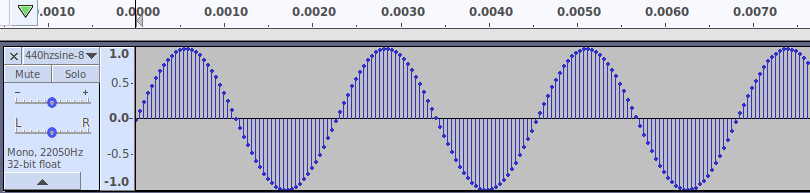
I also plotted e.g. the last 100 bytes, and printed them out to make sure they looked right:

from scipy.io import wavfile
import matplotlib.pyplot as plot

input_sample_rate, wavarray = wavfile.read(file_name)

plot.plot(wavarray[-100:])
plot.show()

print(wavarray[-100:])

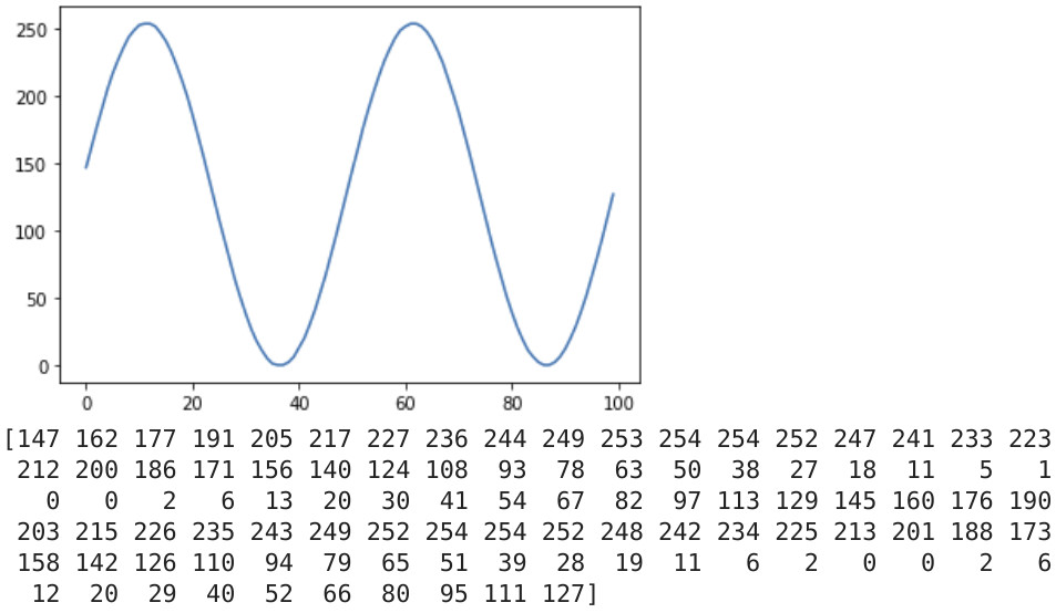
It is really useful to be able to do this at all the stages of data loading, processing and training, just to make sure there aren’t unexpected things happening. Given a not-terribly-large model should be reasonably good at predicting a sine wave, it was also useful for testing the prediction/generation process too.

Loading the data Link to heading

Although being an 8 bit file I could simply read into a bytearray, I opened via scipy.io.wavfile to make it easier to switch to other formats, e.g. 16 bit, at a later date:

from scipy.io import wavfile
samplerate, wavarray = wavfile.read(input_file)

This loads the entire file into a numpy array.

Windowing the data Link to heading

The input to the network (i.e. the features) is a series of samples, and the output (i.e. the label) is the next sample in that series. The is a moving “window” on the data to cover all the samples. Tensorflow can create a special dataset for this. First load the entire series into a Tensorflow dataset:

ds = tf.data.Dataset.from_tensor_slices(wavarray)

Then create a window of window_size, shifting each window by 1 timestep, and trimming the excess at the end to make sure each window is the same shape:

ds = ds.window(window_size + 1, shift=1, drop_remainder=True)

Finally, flatten the data to make it easier to work with, shuffle the data to avoid any sequence bias (with a shuffle_buffer to speed the shuffling), split it into the input (all but last element) and the output (last element), and batch into batch_size:

ds = ds.flat_map(lambda w: w.batch(window_size + 1))
ds = ds.shuffle(shuffle_buffer)
ds = ds.map(lambda w: (w[:-1], w[1:]))
ds = ds.batch(batch_size).prefetch(1)

Splitting into training and validation Link to heading

I simply used the first 80% of the data as training and the last 20% as validation:

def get_split(wavarray):
    split = int(len(wavarray) * 0.8)
    return split

split = get_split(wavarray)
train_array = wavarray[:split]
validate_array = wavarray[split:]

A basic LSTM in Tensorflow, and adding a convolutional layer Link to heading

Basic LSTM Link to heading

I started with a basic model with 2 LSTM layers, like I’d had in the original wav-rnn:

def build_model():
    model = tf.keras.models.Sequential([
        tf.keras.layers.LSTM(256, return_sequences=True),
        tf.keras.layers.LSTM(64),
        tf.keras.layers.Dense(1)
    ])
    return model

A key difference from char-rnn is that my final layer simply outputs one value, whereas char-rnn outputs vocab_size values, i.e. probabilities for each of the 65 possible characters used in the input.

One interesting thing I found is that if you have an LSTM layer as the first layer you can’t use unsigned 8bit (uint8) as the datatype - supported options are dtypes of bfloat16, float16, float32, float64, int32, int64, complex64, complex128. I chose to convert the numpy wavarray from uint8 to int32:

wavarraytype = wavarray.dtype
if wavarraytype == "uint8":
    wavarray = wavarray.astype(np.int32) # convert to int32

The actual numbers in the array stay visibly the same, e.g. it doesn’t convert 128 to 0, but the internal representation changes. At some point I’d like to experiment with other input options (e.g. 16 bit audio) and conversion (e.g. to float32 rather than int32) to see impact on training time, accuracy and so on.

Another interesting point is that I accidentally left return_sequences=True on the second LSTM layer, and even though I had Dense(1) at the end I was getting 64 predictions rather than 1.

Convolutional layer Link to heading

WaveNet’s main innovation is “dilated causal convolution”, which allow longer time series to be covered. I just used an ordinary 1D convolutional layer now, just to keep it simple.

def build_model():
    model = tf.keras.models.Sequential([
        tf.keras.layers.Conv1D(filters=32, kernel_size=5,
            strides=1, padding="causal", activation="relu", input_shape=[None, 1]),
        tf.keras.layers.LSTM(256, return_sequences=True),
        tf.keras.layers.LSTM(64),
        tf.keras.layers.Dense(1)
    ])
    return model

Building and running the model Link to heading

optimizer = tf.keras.optimizers.SGD(lr=1e-6, momentum=0.9)
model = build_model()
model.compile(loss="mse", optimizer=optimizer, metrics=['accuracy'])

checkpoint_prefix = os.path.join(checkpoint_dir, "ckpt_{epoch}")
checkpoint_callback=tf.keras.callbacks.ModelCheckpoint(
    filepath=checkpoint_prefix,
    save_weights_only=True)

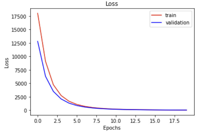
history = model.fit(train_dataset, validation_data=validation_dataset, epochs=epochs, callbacks=[checkpoint_callback])

This gives a reasonable looking plot of training loss and validation loss:

Generating and saving a new wav file Link to heading

To generate new data, I initially took the last window_size of data in the input file, and predicted the next sample. The new prediction was added to the end of the moving window, the first sample removed, and the process repeated, until output_length was reached. This worked okay for the sine waves, but for some real music I found I was generating silence because the last window_size of data in the input file was also silence, so I switched to use the first window_size of data in the input file.

Note the array reshaping - input_wavarray is shape (batch_size, sequence_length/window_size), e.g. shape (1, 300), and it needs to be (batch_size, sequence_length/window_size, series_dimensionality), e.g. shape (1, 300, 1). Note also the casting of dtypes again - the prediction comes back as an int64 but we need to convert to int32 for the input, and the final array needs to be cast back to uint8 for the wav file.

def generate_wav(model, initial_wavarray, output_length):
    generated_wav = []
    progress = common.output_length / 10
    input_wavarray = initial_wavarray
    for i in range(common.output_length):
        prediction_input = input_wavarray[:][np.newaxis]
        prediction_input = tf.expand_dims(prediction_input, axis=-1)
        prediction = model.predict(prediction_input)
        prediction = tf.cast(prediction, tf.int32)
        [predicted_value] = np.array(prediction)[:, 0]
        input_wavarray = np.append(input_wavarray[1:], [predicted_value])
        generated_wav.append(predicted_value)
    print("completed at " + str(datetime.now()))
    return generated_wav

initial_input = wavarray[wavarray.size - window_size:]
generated_wav = np.array(generate_wav(model, initial_input, output_length), dtype=np.uint8)
wavfile.write(output_file, samplerate, generated_wav)

The code for doing this does seem a bit clunky, but I’m not sure there was a more elegant way of doing this, e.g. with a windowed dataset, given data at the end would be unknown at the start.

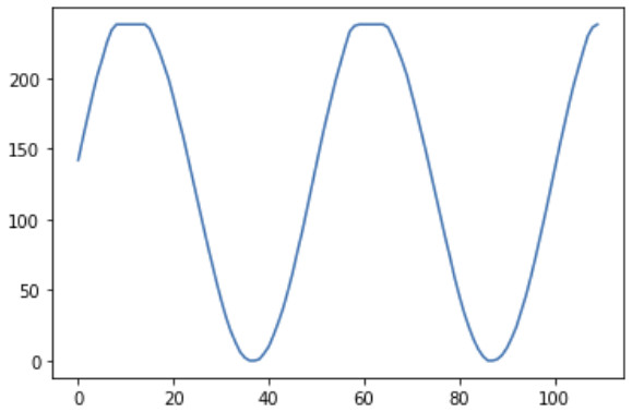
But after just 10 epochs, it generated a reasonable looking sine wave (noting how it picks up where the last 100 bytes shown above left off):

Training with some real music Link to heading

Once I got the end-to-end solution working with a simple sine wave, I moved on to some real music.

I used Beethoven’s 7th Symphony 2nd movement, which is from Wikimedia Commons and licenced under Creative Commons CC BY-SA 3.0 so I believe I can redistribute as long as the licence is referenced.

I know there are ways of doing audio file processing within Python and even Tensorflow itself, but I just did the preprocessing with ffmpeg.

To reduce to an 8-bit unsigned PCM 22,050Hz mono wav file (no file compression etc.):

ffmpeg -i JOHN_MICHEL_CELLO-BEETHOVEN_SYMPHONY_7_Allegretto.ogg -ar 22050 -ac 1 -f wav -acodec pcm_u8 beethoven7th2nd-8bit22050hzmono.wav

Where -ar 22050 sets the audio sampling rate to 22,050, -ac 1 reduces audio channels down to one (mono), -f wav sets the format WAV / WAVE Waveform Audio (see format options via ffmpeg -formats), and -acodec pcm_u8 sets the audio codec to PCM unsigned 8-bit (see codec options via ffmpeg -codecs).

This creates a wav file which will have some headers (-f u8 will create a raw file without headers), so I was able to check specifications after conversion, e.g. via ffmpeg -i beethoven7th2nd-8bit22000hzmono.wav. I also loaded the file into Audacity and gave it a listen just to make sure it hadn’t been corrupted in any way. It sounded pretty hissy being only 8-bit, but was still recognisable.

The command od -vtu1 -An -w1 <file>.wav | sort -n | uniq -c shows that, perhaps unsurprisingly, values for each sample in the file cluster around the 128 mark (which would be 0 in a signed file) and tail off significantly at the top and bottom ends (numbers will be slightly off due to the extra data in the 78 byte file header).

The 10 mins 59 seconds of Beethoven’s 7th Symphony 2nd movement comes to 14,543,712 bytes, which is around 13 times the 1,115,394 bytes of Shakespeare’s complete works, and each sample will have values up to 256 rather than 128 (in practice 65) of Shakespeare, so it is still a lot more data, but the hope was that it was still manageable.

Increasing the network size overfitted the simple sine wave in the first epoch, and started looking like it was overfitting on the longer real music, although colab kept on disconnecting given it was was taking several hours per epoch, so I reduced the size again.

The results Link to heading

When training on the real music, it takes around 2.5 hours per epoch on colab and around 5 hours per epoch on my old GPU. Over the space of 2-3 weeks I’ve been able to complete around 20 epochs, which is unlikely to be sufficient. However, I have still tried the generate function a few times. It takes around 3 hours to generate 10 seconds on colab, and around 6 hours on my GPU. Unfortunately all the generated music so far has been of a consistent pattern, e.g. sounding like silence, clicks or a buzz. I’m wondering if that was because of the decision to have a single output unit - perhaps I should have had 256, similar to the original char-nn, with probabilities assigned to each, and a “temperature” setting to allow experimentation with the randomness. Slightly disappointing though, given all the things I was hearing/imagining in the white noise from the original wav-rnn project 5 years ago.

Future enhancements Link to heading

As noted above, there are a number of additional experiments and opportunities for tuning that can be performed with this solution, e.g.:

• Experiments that can be performed around the input formats, e.g. does converting to 8 bit audio actually help that much?
• Looking into convolutional layers with time dilation as per WaveNet.
• More than just the ultra-basic model and hyperparameter tuning.
• Perhaps make the generation more efficient.

There’s a great guide to things I mostly haven’t done at Recipe for Training Neural Networks.

Looking at the broader aim of generating music, there are also many other areas I’d like to investigate:

• Look at ways of covering significantly longer time series, e.g. with dilated convolutions, or some other higher level abstractions.
• See if it would be possible to blend time domain and frequency domain in some way, e.g. with multiple input layers.
• Try it as a discriminator in a GAN, so I can lean about GANs too.

However, as per the note in the Introduction, given how long it takes to train with even relatively small models, I’m going to put it on hold for a while.